How to Use VLOOKUP in Google Sheets

In this article you’ll learn more about how VLOOKUP works in Google Sheets, and how to use it with a few useful examples.
If you’ve ever used the VLOOKUP function in Excel, then you know just how powerful a function it is. If you’re not sure what VLOOKUP in Google Sheets does, it performs the same way as in Excel.
The VLOOKUP function lets you search the leftmost column of a range in order to return a value from any other column in that same range.
In this article, you’ll learn more about how VLOOKUP works in Google Sheets, and how to use it with a few useful examples.
What Is VLOOKUP in Google Sheets?
Think of VLOOKUP in Google Sheets as a very simple database lookup. When you want information from a database, you need to search for a specific table for a value from one column. Whatever row the search finds a match in that column, you can then look up a value from any other column in that row (or record, in the case of a database).
It works the same way in Google Sheets. The VLOOKUP function has four parameters, with one of them optional. Those parameters are as follows:
- search_key: This is the specific value you’re searching for. It can be a string or a number.
- range: Any range of columns and cells that you want to include in the search.
- index: This is the column number (within the selected range) where you want to get the returned value.
- is_sorted (optional): If set to TRUE, you’re telling the VLOOKUP function that the first column is sorted.
There are a few important things to keep in mind about these parameters.
First, you can select the range as your typing the VLOOKUP function, when you get to the “range” parameter. This makes it easier since you won’t have to remember the correct syntax to define a range.
Second, The “index” needs to be between 1 and the maximum number of columns in your selected range. If you type a number larger than the number of columns in the range, you’ll get an error.
Using VLOOKUP in Google Sheets
Now that you understand how VLOOKUP works, let’s take a look at a few examples.
Example 1: Simple Information Lookup
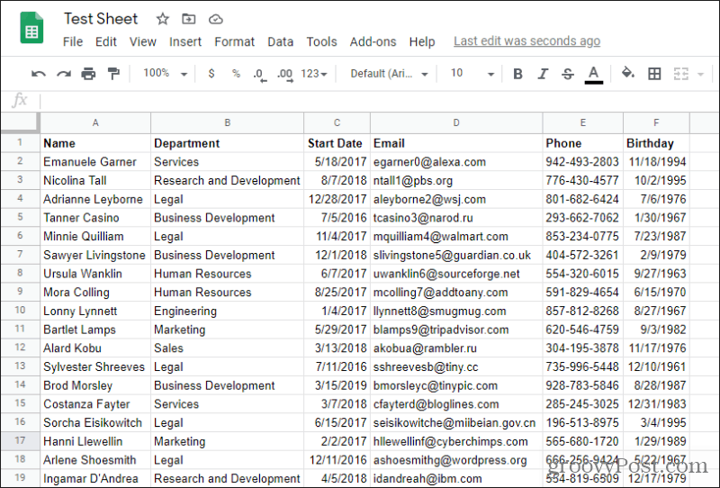
Let’s say you have a list of employees and their associated personal information.
Next, maybe you have Google Sheet with recorded employee sales. Since you calculate their commissions based on their start date, you’ll need a VLOOKUP to grab that from the Start Date field.
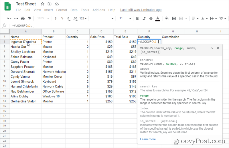
To do this, in the first “Seniority” field, you’ll start typing the VLOOKUP function by typing “=VLOOKUP(“.

The first thing you’ll notice is a help window will appear. If it doesn’t, press the blue “?” icon to the left of the cell.
This help window will tell you what parameter you need to enter next. The first parameter is the search_key, so you just need to select the employee’s name in column A. This will automatically fill in the function with the correct syntax for that cell.
The help window will disappear, but when you type the next comma, it’ll reappear.
As you can see, it shows you that the next parameter you need to fill in is the range you want to search. This will be the employee data lookup range on the other sheet.
So select the tab where the employee data is stored, and highlight the entire range with employee data. Make sure the field you want to search is the leftmost selected column. In this case, that’s “Name”.

You’ll notice the small field with the VLOOKUP function and parameters will float over this sheet while you’re selecting the range. This lets you see how the range is entered into the function while you’re selecting it.
Once you’re done, just type another comma to move on to the next VLOOKUP parameter. You may need to select the original tab you were on to switch back to the results sheet as well.
The next parameter is the index. We know that the Start Date for the employee is the third column in the selected range, so you can just type 3 for this parameter.
Type “FALSE” for the is_sorted parameter since the first column isn’t sorted. Finally, type the closing parenthesis and press Enter.
Now you’ll see the field is filled in with the correct Date Started date for that employee.

Fill the rest of the fields under it and you’re done!
Example 2: Pulling in Data From a Reference Table
In this next example, we’re going to create a reference table of letter grades to pull the correct letter grade for a student’s numerical grade. To set this up you just need to make sure to have a reference table set up somewhere for all of the letter grades.

To look up the correct letter grade in cell C2, just select the cell and type: “=VLOOKUP(B2,$E$1:$F$6,2,TRUE)”
Here’s an explanation of what those parameters mean.
- B2: References the numeric test grade to look up
- $E$1:$F$6: This is the letter grade table, with dollar symbols to keep the range from changing even when you fill the rest of the column
- 2: This references the second column of the lookup table – the Letter Grade
- TRUE: Tells the VLOOKUP function that the scores in the lookup table are sorted
Just fill the rest of column C and you’ll see the correct letter grades get applied.
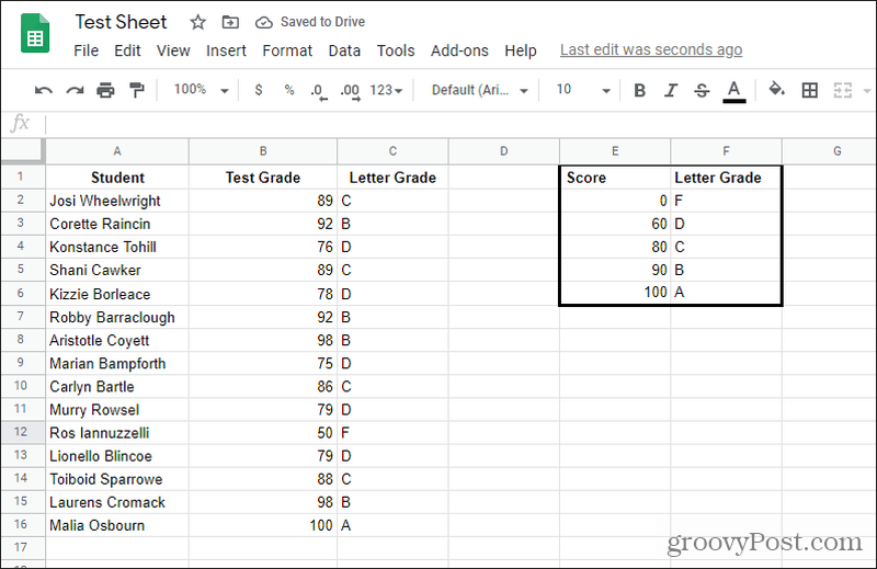
As you can see, the way this works with sorted ranges is the VLOOKUP function grabs the result for the lesser end of the sorted range. So anything from 60 to 79 returns a D, 80 to 89 returns a C, and so on.
Example 3: A VLOOKUP Two-Way Lookup
A final example is using the VLOOKUP function with a nested MATCH function. The use case for this is when you want to search a table by different columns or rows.
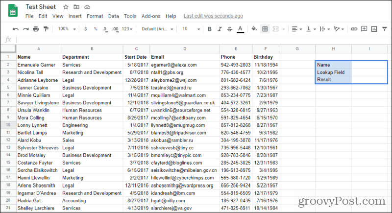
For example, let’s say you have the same employee table as the first example above. You’d like to create a new sheet where you can simply type the employee name, and what information you want to pull up about them. The third cell would then return that information. Sounds cool, right?
You can create this lookup table on the same sheet or a different sheet. It’s up to you. Just create one row for the leftmost column lookup value (the row selection). Create another row for the field you want to search for the result. It should look something like this.
Now, select the empty Result field, and type “=VLOOKUP(I2,A1:F31,MATCH(I3,A1:F1,0),FALSE)” and press Enter.
Before looking at the results, let’s break down how the parameters in this VLOOKUP function work.
- I2: This is the name you’ve typed in the name search field, which VLOOKUP will try to match with a name in the leftmost column of the range.
- A1:F31: This is the entire range of names including all associated information.
- MATCH(I3,A1:F1,0): The match function will use the Lookup Field you’ve entered, find it in the header range, and return the column number. This column number then gets passed to the VLOOKUP function index parameter.
- FALSE: The order of data in the left column isn’t sorted.
Now that you understand how it works, let’s look at the results.

As you can see, by typing the name and the field to return (Email), you can look up any information you like.
You can also use this two-way lookup approach to search any table by both row and column. It’s one of the most useful applications of the VLOOKUP function.
Using VLOOKUP in Google Sheets
Adding the VLOOKUP function to Google Sheets was one of the best things Google could have done. It enhances the usefulness of your spreadsheets and lets you search and even merge multiple sheets.
If you have any issues with the function, many of the troubleshooting tips that work with VLOOKUP in Excel will work for it in Google Sheets as well.