How to Set Up Multiple Conditional Formatting Rules in Google Sheets

You can make all of the important data in your spreadsheets stand out by using multiple conditional formatting rules in Google Sheets.
Conditional formatting in Google Sheets and other spreadsheet applications can help make certain data stand out. You can set up rules that change the appearance of cells when criteria are met. So if you’re working with a lot of data that you want to analyze or track, you may want more than one rule in your sheet.
Here, we’ll show you how easy it is to set up multiple conditional formatting rules in Google Sheets.
Add Another Rule to the Same Cells
Since you’re interested in setting up more than one conditional formatting rule, we’ll assume you have already created one. But you can check out our tutorial for using conditional formatting in Google Sheets for the basics on the feature if needed.
If you want to use another conditional formatting rule for the exact same cells, follow these steps.
- Select the same range of cells or any cell in that range.
- Click Format > Conditional Formatting from the menu.
- When you see your first rule display in the right-hand sidebar, click the rule.
- On the next screen below that rule, click Add another rule.
- Create your next rule and confirm the range of cells in the Apply to range box at the top of the rule.
- Click Done when you finish.
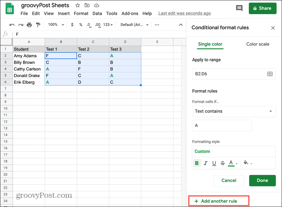

Although not required, it’s best to run a quick test to make sure the new rule works along with the original one.
Adjust the Second Rule Formatting Per the First
When you follow the steps above to set up another rule for the same cells the formatting style used for the first rule will automatically apply to the second. Be sure to change this in the Formatting style box if you want completely different formatting for the second rule.


Add Another Rule to Different Cells
You can also add a conditional formatting rule to different cells on the same sheet.
- Click Format > Conditional Formatting from the menu.
- When the Confirmation Format Rules screen opens in the sidebar, click Add another rule immediately.
- Be sure not to select an existing rule first and then click to Add another rule because that will apply your new rule to the same cells as your first one.


Add the Same Rule to Multiple Cell Ranges
You may have a spreadsheet that’s laid out in a way where you want to apply the exact same conditional formatting rule to multiple ranges of cells. For instance, you might want to highlight empty cells in a range of B2:D6 but not again until range F2:H6. You may have some blank cells for spacing, as an example, and don’t want to highlight those.
- Select the cell range or any cell in the range for the first rule.
- Click Format > Conditional Formatting from the menu.
- When you see your rule display in the right-hand sidebar, click the rule.
- In the Apply to range box, click the icon on the right for Select data range.


- Click Add another range.
- Either type the cell range or drag through it on your sheet. The pop-up will remain open if you do the latter and capture the cells you select.
- Click OK in the pop-up window.
- Then, click Done to save your changes.
You will see your different cell ranges separated by commas in the Apply to range box for that rule.


Remove a Range of Cells
If you use the steps directly above to format multiple cell ranges and decide to remove a range later, this is simple.
- Follow Steps 1 through 4 to open the Select data range pop-up window.
- Hit the Trash can icon next to a range to remove it from the rule.
- Click OK in the pop-up window.
- Then, click Done to save your changes.


Notes on Using Multiple Conditional Formatting Rules
Here are a few things to keep in mind when working with multiple conditional formatting rules in Google Sheets.
- Rules apply to data in the order they are listed. Click, drag, and drop to reorder rules if needed.
- You will only see the rules for a particular sheet in the sidebar. So if you have multiple sheets with rules on each one, select a certain sheet to view its applicable rules.
- If you copy and paste data that has conditional formatting rules associated, those rules will copy and paste as well. This applies to copying and pasting within the same sheet or the same workbook.
- To delete a rule, simply click the Trash can icon next to it on the list.
It’s All About the Rules
Conditional formatting in Google Sheets gives you a terrific way to spot data at a glance. And once you set up a rule, adding others is as easy as a few clicks.
For additional help, take a look at using conditional formatting in Excel too!


