How to Format and Apply Alternating Colors in Google Sheets

You can use alternating colors in Google Sheets to make your data easier to read. See how to format and apply a color scheme between rows of your sheet.
When you create a spreadsheet that holds a lot of data, especially numbers upon numbers, it can be tough to read and analyze. But by applying a basic alternating color scheme, you can make it much simpler. This pattern colors other line of your sheet differently thus making it easier to read.
Here, we’ll show you how to format and apply alternating colors in Google Sheets.
Use Alternating Colors in Google Sheets
Visit the Google Sheets website, sign in, and open the sheet where you want to apply alternating colors.
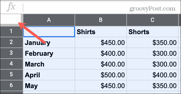
Select the cells you want to apply the color scheme to; this can be a group of columns or rows, range of cells, or the entire sheet. Drag through columns, rows, or cells to select them, or for the whole sheet, click the rectangle on the top left corner where the first column and row meet.

Click Format > Alternating colors from the menu. This displays the Alternating colors sidebar on the right. If you like the defaults that apply to your sheet, you can click Done at the bottom of the sidebar. But if you prefer to make some colorful adjustments, read on!
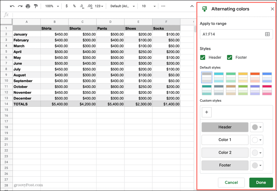

Alternating Color Formatting Options
Use built-in color styles, apply colors to the headers and footers, or create your own color combinations.
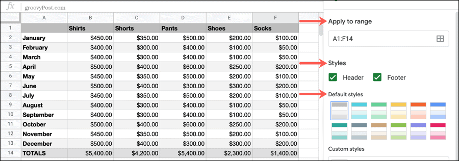
Apply to range: You can adjust your range of cells in the box at the top if necessary. Click inside the box to change the cells or the icon on the right.
Styles: Apply the formatting to the Header and/or the Footer by checking those boxes. This applies a darker shade of the main color to the first and last rows. You can also use a custom color for the header and footer (below).
Default styles: By default, you’ll see gray and white as the alternating colors. But you can use one of the built-in styles you see for a more vibrant visual. Just click one to see how it looks.

Custom styles: Along with the premade color combinations, you can concoct your own. So if you want to get a little creative with your sheet, here’s where you do it.
For each area, Header, Color 1, Color 2, and Footer, click the drop-down to the right. You can then choose any color you like from the palette.


If you have specific colors you want to use, such as hex values, click the plus sign under Custom at the bottom of the palette and enter your color.


Note: Header and Footer custom styles only display when you have those boxes checked in the sidebar.
After making any changes in the Alternating colors, click Done to apply your changes and close the sidebar. You can also click Cancel if you change your mind.
Tips for Alternating Colors in Google Sheets
You can apply different alternating colors to various areas of your sheet. Follow the same steps as above to select the other ranges of cells and choose the formatting. Just be sure to confirm the cells in the Apply to range box and click Done after applying the formatting.


If you set up conditional formatting for your Google Sheets using fill colors, those colors will remain. The surrounding cells will take on the alternating color scheme.
To remove alternating colors later, return to the sidebar by clicking Format > Alternating colors from the menu. Select the cells and click the Remove alternating colors button at the bottom of the sidebar.


Alternating Colors in Google Sheets for Easier Viewing
You can make spreadsheets containing a large amount of data much simpler to view by using simple formatting tricks like alternating colors in Google Sheets.
And if you use Microsoft Excel in addition to Google Sheets, check out how to use alternating colors between rows in Excel too!


