How-To

How to Create Custom Number Formats in Google Sheets

By Sandy Writtenhouse

Updated November 22, 2022

Did you know you can create custom number formats in Google Sheets? This lets you format numbers, dates, and times any way you want.

When you enter numbers in Google Sheets like currencies, dates, times, and decimal numbers, you can format them as such. But if you don’t see the format you want to use in your particular sheet, you can create your own.

We’ll show you how to create custom number formats in Google Sheets. You can start with a built-in format and edit it or create one from scratch; here’s how.

Create a Custom Format Using a Built-In Option

If you want a quick way to create your custom number format, you can start with one of the built-in options. Simply select the one closest to your needs and edit it to fit.

1. Open your spreadsheet in Google Sheets and select the cell(s) containing the number you want to format.
2. Click Format > Number from the menu.
3. In the pop-out menu, move down to More Formats at the bottom of the list.
4. Select either More currencies or More date and time formats per your preference.

When the window appears, you can select an option and make your edits. After customizing the format, just click Apply to use the format in the selected cell(s).

Custom Currencies

For currencies, choose one from the list to begin. In the drop-down box at the top, choose a format option. Then in the box, type in how you want the currency to display with the format you just picked. You’ll see the preview of how the format will appear in the drop-down box.

Custom Dates and Times

For dates and times, do the same by picking one from the list. You have a lot of flexibility in displaying dates and/or times. First, you can use the drop-down list for each element in the date and time to format its display. Second, you can use the drop-down arrow all the way to the right to add even more elements. You can also remove an element by clicking Delete in the drop-down list for it.

Create a Custom Format From Scratch

If you’re using a number other than a currency, date, or time, you can create your custom format from scratch.

1. Open your spreadsheet and select the cell(s) containing the number you want to format.
2. Click Format > Number from the menu.
3. In the pop-out menu, move down to More Formats at the bottom of the list.
4. Select Custom number format.

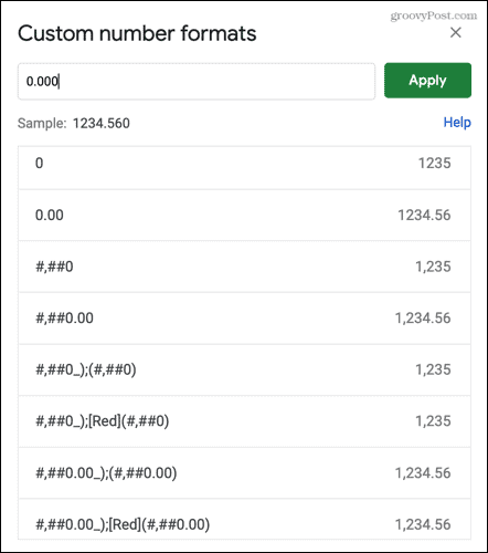
While you can technically start with a built-in option by selecting one from the bottom, you can also type in your own format. Simply enter what you’d like to use in the box at the top. You’ll see a Sample of it directly below, so make your adjustments as needed. Then, click Apply to use the format for the cell(s).

Reuse Your Custom Formats

After you create a custom format using either of the above methods, you can reuse it in the same sheet or any other you open in Google Sheets.

1. Select the cell(s) where you want to apply your custom format.
2. Click Format > Number from the menu.
3. In the pop-out menu, move down to the bottom, and you’ll see those you created directly above More Formats. Simply select one to apply it to the cell(s).

Make Your Own Custom Number Formats in Google Sheets

Having the ability to create custom formats for numbers, dates, times, and even currencies in Google Sheets is a terrific feature. This allows you to use the exact type you need.

For more, take a look at how to use conditional formatting for common tasks or create multiple formatting rules in Google Sheets.